Nonlinear model predictive control (regulation) in MATLAB with YALMIP

In this post we will attempt to create nonlinear model predictive control (MPC) code for the regulation problem (i.e., steering the state to a fixed equilibrium and keeping it there) in MATLAB using YALMIP. We will need MATLAB, YALMIP¹ (a free Octave/MATLAB toolbox for optimization modeling), and Ipopt² (for solving the resulting nonlinear optimization problems). You can download the code created in this post here: regulation_NMPC_YALMIP.m. The same code with “optimize” calls instead of the “optimizer” object, which might be useful for easier debugging or seeing more details, can be found here: regulation_NMPC_YALMIP_mod.m.

Note: For MPC code with high computational efficiency, use of either CasADi³ or MPCTools⁴ is recommended (see, e.g., here).

We consider the following nonlinear MPC formulation:

\[\begin{aligned} \text{minimize} & \quad \int_{t}^{t+T_p}{l(x(\tau),u(\tau))d\tau} + V_f(x(t+T_p)) \\ \text{subject to} & \quad x(t) = \hat{x}(t) \\ & \quad \text{for } \tau \in [t, t+T_p]: \\ & \qquad \dot{x}(\tau) = f(x(\tau),u(\tau)) \\ & \qquad x_{\text{min}} \leq x(\tau) \leq x_{\text{max}} \\ & \qquad u_{\text{min}} \leq u(\tau) \leq u_{\text{max}} \\ & \quad e_f(x(t+T_p)) \leq 0, \end{aligned}\]

where \(T_p\) is the prediction horizon (in time units), \(l(\cdot)\) is the stage cost, \(x \in \mathbb{R}^{n_x}\) is the state vector, \(u \in \mathbb{R}^{n_u}\) is the control input vector, \(V_f(\cdot)\) is the terminal cost, \(\hat{x}(t)\) is the measurement, \(f(\cdot)\) is the dynamics, \(x_{\text{min}}\) and \(x_{\text{max}}\) are state constraints, \(u_{\text{min}}\) and \(u_{\text{max}}\) are control input constraints, while \(e_f\) is the terminal state constraint.

As an example, we take the following two dimensional system⁵:

\[\begin{aligned} \dot{x}_1(t) & = x_2(t) + u(t) \left( \mu + \left( 1 - \mu \right)x_1(t) \right) \\ \dot{x}_2(t) & = x_1(t) + u(t) \left( \mu - 4 \left( 1 - \mu \right)x_2(t)\right), \end{aligned}\]

where \(x_1(t) \in \mathbb{R}\) and \(x_2(t) \in \mathbb{R}\) are the state variables, \(u(t) \in \mathbb{R}\) is the control input, and \(\mu\) is a parameter we assume to be \(0.5\) here. In compact form we can write the dynamics as \(\dot{x}(t)=f(x(t),u(t))\), which we can define in code as follows:

function dxdt = define_dynamics(t,x,u)
    
    mu = 0.5;
    
    dxdt = [x(2) + u*(mu + (1-mu)*x(1)); ...
        x(1) + u*(mu - 4*(1-mu)*x(2))];
    
end

We specify various parameters and pre-allocate memory for the signals as follows:

function d = build_setup(d)
    
    % state constraints
    d.p.x_min = -Inf;
    d.p.x_max = Inf;
    
    % control input constraints
    d.p.u_min = -2;
    d.p.u_max = 2;
    
    % NMPC prediction horizon (in number of time steps)
    d.p.N_NMPC = 15;
    
    % sampling time (in time units)
    d.p.T = 0.1;
    
    % number of state variables
    d.p.n_x = 2;
    
    % number of control inputs
    d.p.n_u = 1;
    
    % simulation length (in number of time steps)
    d.p.t_final = 120;
    
    % pre-allocate memory
    d.s.x = NaN(d.p.n_x,d.p.t_final);
    d.s.u = NaN(d.p.n_u,d.p.t_final);
    
    % set initial state
    % (d.p.x0 is an argument of the main function)
    d.s.x(:,1) = d.p.x0;
    
    % state constraints vector
    d.p.x_min_v = d.p.x_min*ones(d.p.n_x,1);
    d.p.x_max_v = d.p.x_max*ones(d.p.n_x,1);
    
    % control input constraints vector
    d.p.u_min_v = d.p.u_min*ones(d.p.n_u,1);
    d.p.u_max_v = d.p.u_max*ones(d.p.n_u,1);
    
    % weighting matrices of stage cost
    d.p.Q = 0.5*eye(d.p.n_x);
    d.p.R = eye(d.p.n_u);
    
    % weighting matrix and bound for terminal cost and constraint
    d.p.P = [16.5926 11.5926;11.5926 16.5926];
    d.p.alpha = 0.7;
    
end

Here the use of -Inf and Inf indicates that the state is unconstrained, while the control input is constrained as \(-2 \leq u(t) \leq 2\).

We can create a RK4 integrator, for use as both simulation model (to act as the plant within simulation) and prediction model (for the MPC predictions) as follows:

function x_plus = F(f,x,u,h)
    
    % create RK4 integrator
    k1 = f(0,x,u);
    k2 = f(0,x+(h/2).*k1,u);
    k3 = f(0,x+(h/2).*k2,u);
    k4 = f(0,x+h.*k3,u);
    x_plus = x + (h/6).*(k1+2*k2+2*k3+k4);
    
end

We can build the nonlinear MPC with the following parts:

a) Define the control input and state trajectories as decision variables

% define control inputs as decision variables
u = sdpvar(d.p.n_u,d.p.N_NMPC,'full');

% define states as decision variables
x = sdpvar(d.p.n_x,d.p.N_NMPC+1,'full');

b) Initialize objective function and constraints:

% initialize objective function
obj = 0;

% initialize constraints
con = [];

c) Use the RK4 integrator to form the predicted state trajectory

for k = 1:d.p.N_NMPC
    
    % ensure continuity of state trajectory
    % (i.e., direct multiple shooting)
    con = [con, x(:,k+1) == F(@define_dynamics, x(:,k), u(:,k), d.p.T)];
    
end

d) Considering a stage cost \(l(\cdot)\) in line with the regulation problem (which thus expresses the objective of keeping the state \(x(t)\) at the origin while also penalizing nonzero control inputs) as follows

\[\begin{equation} l(x(t),u(t)) = \left\lVert x(t) \right\rVert^2_Q + \left\lVert u(t) \right\rVert^2_R, \end{equation}\]

with

\[\begin{equation} Q = \begin{bmatrix} 0.5 ~ 0 \\ 0 ~ 0.5 \end{bmatrix} \qquad R = 1, \end{equation}\]

we create the objective function by summing over the stage costs

for k = 1:d.p.N_NMPC
    
    % add stage cost to objective function
    obj = obj + x(:,k)'*d.p.Q*x(:,k) + u(:,k)'*d.p.R*u(:,k);
    
end

e) Define control input and state constraints:

for k = 1:d.p.N_NMPC
    
    % control input constraints
    con = [con, d.p.u_min_v <= u(:,k) <= d.p.u_max_v];
    
    % state constraints
    con = [con, d.p.x_min_v <= x(:,k) <= d.p.x_max_v];
    
end

f) Considering terminal cost \(V_f\) and terminal state constraint \(e_f\) (as, for example, required by the quasi-infinite horizon nonlinear MPC method⁵ for guaranteeing closed-loop stability) as follows:

\[\begin{align} V_f & = \left\lVert x \right\rVert^2_P \\ e_f & = x^T P x - \alpha \leq 0, \end{align}\]

with

\[\begin{equation} P = \begin{bmatrix} 16.5926 ~ 11.5926 \\ 11.5926 ~ 16.5926 \end{bmatrix} \qquad \alpha = 0.7, \end{equation}\]

we add the terminal cost and constraint to the MPC formulation as follows:

% add terminal cost to objective function
obj = obj + x(:,d.p.N_NMPC+1)'*d.p.P*x(:,d.p.N_NMPC+1);

% terminal constraint
con = [con, x(:,d.p.N_NMPC+1)'*d.p.P*x(:,d.p.N_NMPC+1) <= d.p.alpha];

g) We can finally create a controller object as a YALMIP optimizer object as follows:

% define optimization settings
ops = sdpsettings;
ops.verbose = 0; % configure level of info solver displays
ops.solver = 'ipopt'; % choose solver

% configure the outputs of the controller object
solutions_out = [u(:);x(:)];

% create MPC controller object
d.c.controller = optimizer(con,obj,ops,x(:,1),solutions_out);

Furthermore, for calling the NMPC during simulation, we need

function d = solve_NMPC(d,t)
    
    tic_c = tic;
    
    % solve NMPC problem
    % (by calling the MPC controller object)
    sol_t = d.c.controller{d.s.x(:,t)};
    
    % record CPU time
    d.s.CPU_time(t,1) = toc(tic_c);
    
    % extract the control input trajectory
    % from the solution of MPC optimization problem
    u_t = sol_t(1:d.p.N_NMPC)';
    
    % record the predicted state trajectory
    % for the first time step
    if t == 1
        
        % extract the state trajectory
        % from the solution of MPC optimization problem
        x_t = reshape(sol_t(d.p.N_NMPC+1:end),[d.p.n_x d.p.N_NMPC+1]);
        
        d.p.x_NMPC_t_1 = x_t;
        
    end
    
    % assign first element of the solution to the NMPC
    % problem as the control input at time t
    d.s.u(:,t) = u_t(:,1);
    
end

and to simulate the dynamical system we need

function d = evolve_dynamics(d,t)
    
    d.s.x(:,t+1) = ...
        F(@define_dynamics, d.s.x(:,t), d.s.u(:,t), d.p.T);
    
end

All pieces are integrated in the function regulation_NMPC_YALMIP.m, which can be run by executing the command

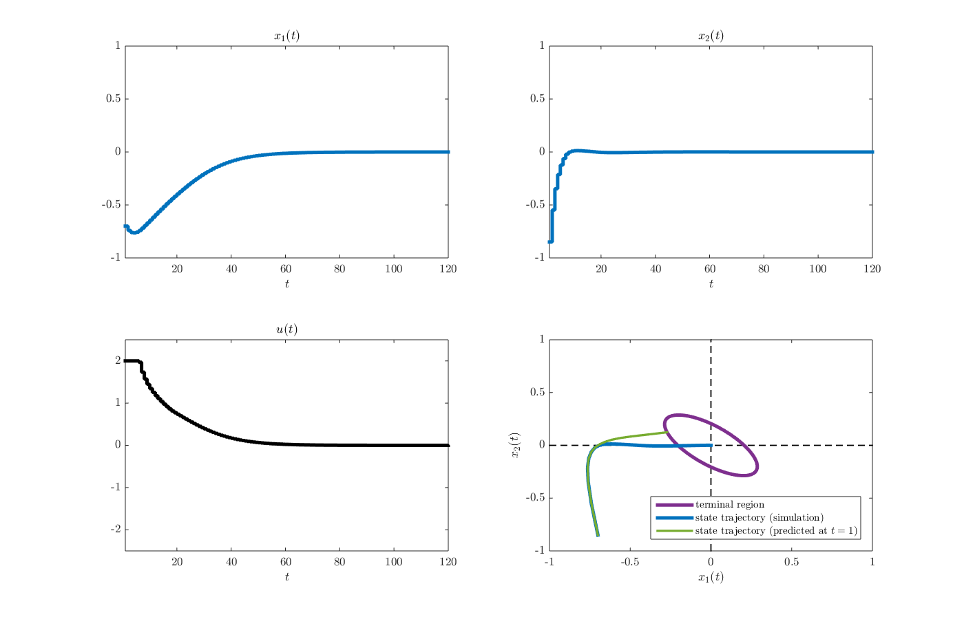
d = regulation_NMPC_YALMIP(-0.7,-0.85)

from the MATLAB command window. The arguments here (i.e., \(-0.7\) and \(-0.85\)) are elements of the initial state vector. After the simulation is finished, the results should appear as a structure named d in the MATLAB workspace. A figure summarizing the results, including the state and control input trajectories, can be produced using the function plot_results_regulation_NMPC.m by executing the command

plot_results_regulation_NMPC(d)

from the MATLAB command window. The resulting figure is given below.

regulation NMPC with YALMIP, results

Löfberg, J. (2004, September). YALMIP: A toolbox for modeling and optimization in MATLAB. In 2004 IEEE international conference on robotics and automation (pp. 284-289). ↩
Wächter, A., & Biegler, L. T. (2006). On the implementation of an interior-point filter line-search algorithm for large-scale nonlinear programming. Mathematical programming, 106(1), 25-57. ↩
Andersson, J. A., Gillis, J., Horn, G., Rawlings, J. B., & Diehl, M. (2018). CasADi: a software framework for nonlinear optimization and optimal control. Mathematical Programming Computation, 1-36. ↩
Risbeck, M. J., & Rawlings, J. B. (2016). MPCTools: Nonlinear model predictive control tools for CasADi. ↩
Chen, H., & Allgöwer, F. (1998). A Quasi-Infinite Horizon Nonlinear Model Predictive Control Scheme with Guaranteed Stability. Automatica, 34(10), 1205-1217. ↩ ↩²

Işık İlber Sırmatel

Nonlinear model predictive control (regulation) in MATLAB with YALMIP

Leave a Comment

You May Also Enjoy

A Coverage Control-Based Idle Vehicle Rebalancing Approach for Autonomous Mobility-on-Demand Systems

Nonlinear model predictive control of large-scale urban road networks via average speed control

Idle-vehicle rebalancing coverage control for ride-sourcing systems

Modeling, estimation, and control in large-scale urban road networks with remaining travel distance dynamics