
Nonlinear model predictive control (regulation) in MATLAB with MPCTools
In this post we will attempt to create nonlinear model predictive control (MPC) code for the regulation problem (i.e., steering the state to a fixed equilibrium and keeping it there) in MATLAB using MPCTools. We will need MATLAB (version R2015b or higher), MPCTools1 (a free Octave/MATLAB toolbox for nonlinear MPC), and CasADi2 (version 3.1 or higher) (a free Python/MATLAB toolbox for nonlinear optimization and numerical optimal control). MPCTools calls Ipopt3 for solving the resulting nonlinear optimization problems. You can download the code created in this post here: regulation_NMPC_MPCTools.m.
We consider the following nonlinear MPC formulation:
\[\begin{aligned} \text{minimize} & \quad \int_{t}^{t+T_p}{l(x(\tau),u(\tau))d\tau} + V_f(x(t+T_p)) \\ \text{subject to} & \quad x(t) = \hat{x}(t) \\ & \quad \text{for } \tau \in [t, t+T_p]: \\ & \qquad \dot{x}(\tau) = f(x(\tau),u(\tau)) \\ & \qquad x_{\text{min}} \leq x(\tau) \leq x_{\text{max}} \\ & \qquad u_{\text{min}} \leq u(\tau) \leq u_{\text{max}} \\ & \quad e_f(x(t+T_p)) \leq 0, \end{aligned}\]where \(T_p\) is the prediction horizon (in time units), \(l(\cdot)\) is the stage cost, \(x \in \mathbb{R}^{n_x}\) is the state vector, \(u \in \mathbb{R}^{n_u}\) is the control input vector, \(V_f(\cdot)\) is the terminal cost, \(\hat{x}(t)\) is the measurement, \(f(\cdot)\) is the dynamics, \(x_{\text{min}}\) and \(x_{\text{max}}\) are state constraints, \(u_{\text{min}}\) and \(u_{\text{max}}\) are control input constraints, while \(e_f\) is the terminal state constraint.
As an example, we take the following two dimensional system4:
\[\begin{aligned} \dot{x}_1(t) & = x_2(t) + u(t) \left( \mu + \left( 1 - \mu \right)x_1(t) \right) \\ \dot{x}_2(t) & = x_1(t) + u(t) \left( \mu - 4 \left( 1 - \mu \right)x_2(t)\right), \end{aligned}\]where \(x_1(t) \in \mathbb{R}\) and \(x_2(t) \in \mathbb{R}\) are the state variables, \(u(t) \in \mathbb{R}\) is the control input, and \(\mu\) is a parameter we assume to be \(0.5\) here. In compact form we can write the dynamics as \(\dot{x}(t)=f(x(t),u(t))\), which we can define in code as follows:
function dxdt = define_dynamics(x, u)

    dxdt = [x(2) + u*(0.5 + 0.5*x(1));
        x(1) + u*(0.5 - 2*x(2))];

end
We specify various parameters and pre-allocate memory for the signals as follows:
function d = build_setup(d)

    % state constraints
    d.p.x_min = -Inf;
    d.p.x_max = Inf;

    % control input constraints
    d.p.u_min = -2;
    d.p.u_max = 2;

    % NMPC prediction horizon (in number of time steps)
    d.p.N_NMPC = 15;

    % sampling time (in time units)
    d.p.T = 0.1;

    % number of state variables
    d.p.n_x = 2;

    % number of control inputs
    d.p.n_u = 1;

    % simulation length (in number of time steps)
    d.p.t_final = 120;

    % pre-allocate memory
    d.s.x = NaN(d.p.n_x,d.p.t_final);
    d.s.u = NaN(d.p.n_u,d.p.t_final);

    % set initial state
    % (d.p.x0 is an argument of the main function)
    d.s.x(:,1) = d.p.x0;

    % state constraints vector
    d.p.x_min_v = d.p.x_min*ones(d.p.n_x,1);
    d.p.x_max_v = d.p.x_max*ones(d.p.n_x,1);

    % control input constraints vector
    d.p.u_min_v = d.p.u_min*ones(d.p.n_u,1);
    d.p.u_max_v = d.p.u_max*ones(d.p.n_u,1);

    % weighting matrices of stage cost
    d.p.Q = 0.5*eye(d.p.n_x);
    d.p.R = eye(d.p.n_u);

    % weighting matrix and bound for terminal cost and constraint
    d.p.P = [16.5926 11.5926;11.5926 16.5926];
    d.p.alpha = 0.7;

    global Q R P alpha
    Q = d.p.Q;
    R = d.p.R;
    P = d.p.P;
    alpha = d.p.alpha;

end
Here the use of -Inf and Inf indicates that the state is unconstrained, while the control input is constrained as \(-2 \leq u(t) \leq 2\).
We can create a simulator object, that will act as the plant within the simulation, as follows:
function d = create_simulator(d)

    d.c.simulator = ...
        d.c.mpc.getCasadiIntegrator(@define_dynamics, ...
        d.p.T, [d.p.n_x, d.p.n_u], {'x', 'u'});

end
Here the arguments are the dynamics \(f(\cdot)\), sampling time \(T\), and dimensions of the state and the control input. Note that, in the code, the structure d is the main structure containing everything, while the fields of d, namely p, s, and c contain parameters, signals, and controller objects, respectively.
We can build the nonlinear MPC with the following parts:
a) Import the dynamics \(f(\cdot)\):
ode_casadi_NMPC = d.c.mpc.getCasadiFunc(...
        @define_dynamics, ...
        [d.p.n_x, d.p.n_u], ...
        {'x', 'u'});
b) Specify how \(f(\cdot)\) should be discretized in time to get \(x(k+1) = F(x(k),u(k))\) by creating the function \(F(\cdot)\):
F = d.c.mpc.getCasadiFunc(...
        ode_casadi_NMPC, ...
        [d.p.n_x, d.p.n_u], ...
        {'x', 'u'}, ...
        'rk4', true(), ...
        'Delta', d.p.T);
Here the arguments are dimensions of the state and control input, whether to use an explicit Runge-Kutta method or not, via setting 'rk4' either true or false, and the timestep 'Delta'.
c) Considering a stage cost \(l(\cdot)\) in line with the regulation problem (which thus expresses the objective of keeping the state \(x(t)\) at the origin while also penalizing nonzero control inputs) as follows
\[\begin{equation} l(x(t),u(t)) = \left\lVert x(t) \right\rVert^2_Q + \left\lVert u(t) \right\rVert^2_R, \end{equation}\]with
\[\begin{equation} Q = \begin{bmatrix} 0.5 ~ 0 \\ 0 ~ 0.5 \end{bmatrix} \qquad R = 1, \end{equation}\]we create \(l(\cdot)\) in code as follows:
function l = define_stage_cost(x,u)

    global Q R

    l = x'*Q*x + u'*R*u;

end
d) Considering terminal cost \(V_f\) and terminal state constraint \(e_f\) (as, for example, required by the quasi-infinite horizon nonlinear MPC method4 for guaranteeing closed-loop stability) as follows:
\[\begin{align} V_f & = \left\lVert x \right\rVert^2_P \\ e_f & = x^T P x - \alpha \leq 0, \end{align}\]with
\[\begin{equation} P = \begin{bmatrix} 16.5926 ~ 11.5926 \\ 11.5926 ~ 16.5926 \end{bmatrix} \qquad \alpha = 0.7, \end{equation}\]we create \(V_f(\cdot)\) and \(e_f(\cdot)\) in code as follows:
function Vf = define_terminal_cost(x)

    global P

    Vf = x'*P*x;

end
function ef = define_terminal_constraint(x)

    global P alpha

    ef = x'*P*x - alpha;

end
We can finally create the nonlinear model predictive controller as follows:
function d = create_NMPC(d)

    % import dynamics
    ode_casadi_NMPC = d.c.mpc.getCasadiFunc(...
        @define_dynamics, ...
        [d.p.n_x, d.p.n_u], ...
        {'x', 'u'});

    % discretize dynamics in time
    F = d.c.mpc.getCasadiFunc(...
        ode_casadi_NMPC, ...
        [d.p.n_x, d.p.n_u], ...
        {'x', 'u'}, ...
        'rk4', true(), ...
        'Delta', d.p.T);

    % define stage cost
    l = d.c.mpc.getCasadiFunc(@define_stage_cost, ...
        [d.p.n_x, d.p.n_u], ...
        {'x', 'u'});

    % define terminal cost
    Vf = d.c.mpc.getCasadiFunc(@define_terminal_cost, ...
        d.p.n_x, {'x'}, {'Vf'});

    % define terminal state constraint
    ef = d.c.mpc.getCasadiFunc(@define_terminal_constraint, ...
        d.p.n_x, {'x'}, {'ef'});

    % define NMPC arguments
    commonargs.l = l;
    commonargs.lb.x = d.p.x_min_v;
    commonargs.ub.x = d.p.x_max_v;
    commonargs.lb.u = d.p.u_min_v;
    commonargs.ub.u = d.p.u_max_v;
    commonargs.Vf = Vf;
    commonargs.ef = ef;

    % define NMPC problem dimensions
    N.x = d.p.n_x; % state dimension
    N.u = d.p.n_u; % control input dimension
    N.t = d.p.N_NMPC; % time dimension (i.e., prediction horizon)

    % create NMPC solver
    d.c.solvers.NMPC = d.c.mpc.nmpc(...
        'f', F, ... % dynamics (discrete-time)
        'N', N, ... % problem dimensions
        'Delta', d.p.T, ... % timestep
        'timelimit', 1, ... % solver time limit (in seconds)
        '**', commonargs); % arguments

end
Furthermore, for calling the NMPC during simulation, we need
function d = solve_NMPC(d,t)

    % set state at time t as NMPC initial state
    d.c.solvers.NMPC.fixvar('x', 1, d.s.x(:,t));

    tic_c = tic;

    % solve NMPC problem
    d.c.solvers.NMPC.solve();

    % record CPU time
    d.s.CPU_time(t,1) = toc(tic_c);

    % assign first element of the solution to the NMPC
    % problem as the control input at time t
    d.s.u(:,t) = d.c.solvers.NMPC.var.u(:,1);

    % record the predicted state trajectory
    % for the first time step
    if t == 1

        d.p.x_NMPC_t_1 = d.c.solvers.NMPC.var.x;

    end

end
and to simulate the dynamical system we need
function d = evolve_dynamics(d,t)

    d.s.x(:,t+1) = ...
        full(d.c.simulator(d.s.x(:,t), d.s.u(:,t)));

end
All pieces are integrated in the function regulation_NMPC_MPCTools.m, which can be run by executing the command
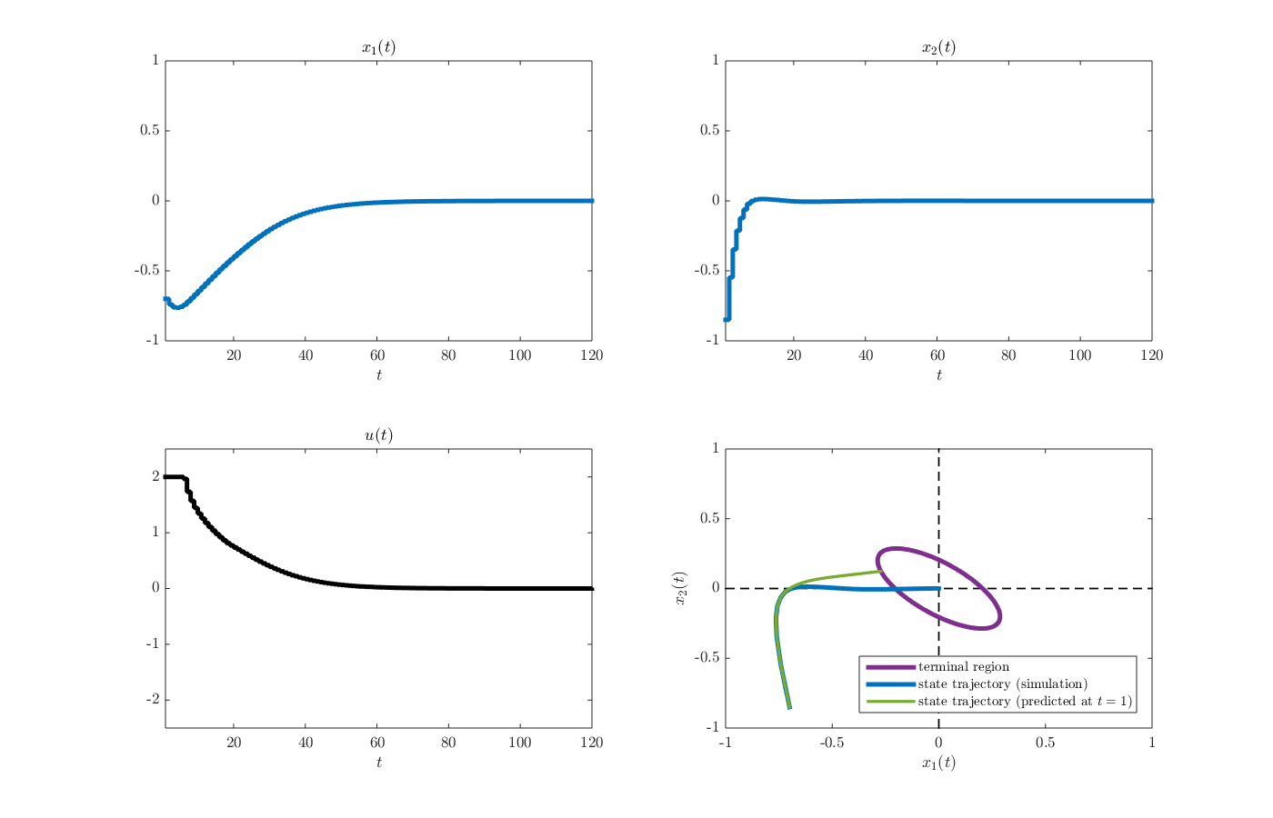
d = regulation_NMPC_MPCTools(-0.7,-0.85)
from the MATLAB command window. The arguments here (i.e., \(-0.7\) and \(-0.85\)) are elements of the initial state vector. After the simulation is finished, the results should appear as a structure named d in the MATLAB workspace. A figure summarizing the results, including the state and control input trajectories, can be produced using the function plot_results_regulation_NMPC.m by executing the command
plot_results_regulation_NMPC(d)
from the MATLAB command window. The resulting figure is given below.
-
Risbeck, M. J., & Rawlings, J. B. (2016). MPCTools: Nonlinear model predictive control tools for CasADi. ↩
-
Andersson, J. A., Gillis, J., Horn, G., Rawlings, J. B., & Diehl, M. (2018). CasADi: a software framework for nonlinear optimization and optimal control. Mathematical Programming Computation, 1-36. ↩
-
Wächter, A., & Biegler, L. T. (2006). On the implementation of an interior-point filter line-search algorithm for large-scale nonlinear programming. Mathematical programming, 106(1), 25-57. ↩
-
Chen, H., & Allgöwer, F. (1998). A Quasi-Infinite Horizon Nonlinear Model Predictive Control Scheme with Guaranteed Stability. Automatica, 34(10), 1205-1217. ↩ ↩2
Leave a Comment