
Nonlinear moving horizon estimation in MATLAB with MPCTools
In this post we will attempt to create nonlinear moving horizon estimation (MHE) code in MATLAB using MPCTools. We will need MATLAB (version R2015b or higher), MPCTools1 (a free Octave/MATLAB toolbox for nonlinear MPC), and CasADi2 (version 3.1 or higher) (a free Python/MATLAB toolbox for nonlinear optimization and numerical optimal control). MPCTools calls Ipopt3 for solving the resulting nonlinear optimization problems. You can download the code created in this post here: NMHE_MPCTools.m.
We consider the following nonlinear MHE formulation:
\[\begin{aligned} \text{minimize} & \quad \int_{t-T_e}^{t}{\left\lVert w(\tau) \right\rVert^2_Q + \left\lVert v(\tau) \right\rVert^2_R} d\tau \\ \text{subject to} & \quad \text{for } \tau \in [t-T_e, t]: \\ & \qquad \dot{x}(\tau) = f(x(\tau)) + w(\tau) \\ & \qquad y(\tau) = h(x(\tau)) + v(\tau) \\ & \qquad x_{\text{min}} \leq x(\tau) \leq x_{\text{max}}, \end{aligned}\]where \(T_e\) is the estimation horizon (in time units), \(w \in \mathbb{R}^{n_w}\) is the process noise, \(v \in \mathbb{R}^{n_v}\) is the measurement noise, \(Q\) and \(R\) are inverse covariance matrices of the process and measurement noise, respectively, \(x \in \mathbb{R}^{n_x}\) is the state, \(f(\cdot)\) is the dynamics, \(y \in \mathbb{R}^{n_y}\) is the measurement, while \(x_{\text{min}}\) and \(x_{\text{max}}\) are state constraints.
As an example, we take the van der Pol oscillator:
\[\begin{aligned} \dot{x}_1(t) & = x_2(t) + w_1(t)\\ \dot{x}_2(t) & = \mu \left( 1 - x_1^2(t) \right)x_2(t) - x_1(t) + w_2(t), \end{aligned}\]where \(x_1(t) \in \mathbb{R}\) and \(x_2(t) \in \mathbb{R}\) are the state variables, \(w_1(t) \in \mathbb{R}\) and \(w_2(t) \in \mathbb{R}\) are the process noise terms, and \(\mu\) is a parameter we assume to be \(1\) here. In compact form we can write the dynamics as \(\dot{x}(t)=f(x(t),w(t))\), which we can define in code as follows:
function dxdt = define_dynamics(x, w)

    dxdt = [x(2) + w(1);
        (1-(x(1)^2))*x(2) - x(1) + w(2)];

end
We specify various parameters and pre-allocate memory for the signals as follows:
function d = build_setup(d)

    % state constraints
    d.p.x_min = -Inf;
    d.p.x_max = Inf;

    % NMHE estimation horizon (in number of time steps)
    d.p.N_NMHE = 15;

    % sampling time (in time units)
    d.p.T = 0.1;

    % number of state variables
    d.p.n_x = 2;

    % number of process noise variables
    d.p.n_w = 2;

    % number of measurements
    d.p.n_y = 2;

    % number of measurement noise variables
    d.p.n_v = 2;

    % simulation length (in number of time steps)
    d.p.t_final = 120;

    % pre-allocate memory
    d.s.x = NaN(d.p.n_x,d.p.t_final); % state
    d.s.x_hat = NaN(d.p.n_x,d.p.t_final); % state estimate
    d.s.y = NaN(d.p.n_y,d.p.t_final); % measurement
    d.s.CPU_time = NaN(d.p.t_final,1); % NMHE CPU time

    % set initial state
    d.s.x(:,1) = d.p.x0;

    % process noise standard deviations
    d.p.sigma_w = [0.1 0.1]';

    % measurement noise standard deviations
    d.p.sigma_v = [1 1]';

    % process noise covariance
    d.p.Sigma_w = diag(d.p.sigma_w.^2);

    % process noise inverse covariance
    d.p.Q = d.c.mpc.spdinv(d.p.Sigma_w);

    % measurement noise covariance
    d.p.Sigma_v = diag(d.p.sigma_v.^2);

    % measurement noise inverse covariance
    d.p.R = d.c.mpc.spdinv(d.p.Sigma_v);

    % set random number generator seed to 0
    rng(0)

    % create process noise signal
    d.s.w = diag(d.p.sigma_w)*randn(d.p.n_w, d.p.t_final);

    % create measurement noise signal
    d.s.v = diag(d.p.sigma_v)*randn(d.p.n_v, d.p.t_final);

    % state constraints vector
    d.p.x_min_v = d.p.x_min*ones(d.p.n_x,1);
    d.p.x_max_v = d.p.x_max*ones(d.p.n_x,1);

end
We can create a simulator object, that will act as the plant within the simulation, as follows:
function d = create_simulator(d)

    d.c.simulator = ...
        d.c.mpc.getCasadiIntegrator(@define_dynamics, ...
        d.p.T, [d.p.n_x, d.p.n_w], {'x', 'w'});

end
Here the arguments are the dynamics \(f(\cdot)\), sampling time \(T\), and dimensions of the state and the process noise. Note that, in the code, the structure d is the main structure containing everything, while the fields of d, namely p, s, and c contain parameters, signals, and controller/estimator objects, respectively.
We can build the nonlinear MHE as follows:
function d = create_NMHE(d)

    % import dynamics
    ode_casadi_NMHE = d.c.mpc.getCasadiFunc(...
        @define_dynamics, ...
        [d.p.n_x, d.p.n_w], ...
        {'x', 'w'});

    % discretize dynamics in time
    F = d.c.mpc.getCasadiFunc(...
        ode_casadi_NMHE, ...
        [d.p.n_x, d.p.n_w], ...
        {'x', 'w'}, ...
        'rk4', true(), ...
        'Delta', d.p.T);

    % define stage cost
    l = d.c.mpc.getCasadiFunc(@(w, v) ...
        w'*d.p.Q*w + v'*d.p.R*v, ...
        [d.p.n_w, d.p.n_v], ...
        {'w', 'v'});

    % define measurement equation
    d.c.h = d.c.mpc.getCasadiFunc(@(x) x, ...
        d.p.n_x, {'x'}, {'H'});

    % define NMHE arguments
    commonargs.l = l;
    commonargs.h = d.c.h;
    commonargs.y = zeros(d.p.n_y,d.p.N_NMHE+1);
    commonargs.lb.x = repmat(d.p.x_min_v,1,d.p.N_NMHE+1);
    commonargs.ub.x = repmat(d.p.x_max_v,1,d.p.N_NMHE+1);

    % define NMHE problem dimensions
    N.x = d.p.n_x; % state dimension
    N.w = d.p.n_w; % process noise dimension
    N.y = d.p.n_y; % measurement dimension
    N.t = d.p.N_NMHE; % time dimension (i.e., estimation horizon)

    % create NMHE solver
    d.c.solvers.NMHE = d.c.mpc.nmhe(...
        'f', F, ...
        'N', N, ...
        '**', commonargs, ...
        'priorupdate', 'none');

end
Furthermore, for calling the NMHE during simulation, we need
function d = solve_NMHE(d,t)

    % record new measurement
    d.c.solvers.NMHE.newmeasurement(d.s.y(:,t));

    tic_e = tic;

    % solve NMHE problem
    d.c.solvers.NMHE.solve();

    % record CPU time
    d.s.CPU_time(t,1) = toc(tic_e);

    % assign last element of the state trajectory (found
    % as NMHE solution) as the state estimate at time t
    d.s.x_hat(:,t) = d.c.solvers.NMHE.var.x(:,end);

end
and to simulate the dynamical system we need
function d = evolve_dynamics(d,t)

    if t < d.p.t_final

        d.s.x(:,t+1) = ...
            full(d.c.simulator(d.s.x(:,t), d.s.w(:,t)));

    end

end
All pieces are integrated in the function NMHE_MPCTools.m, which can be run by executing the command
d = NMHE_MPCTools(1.5,1.5)
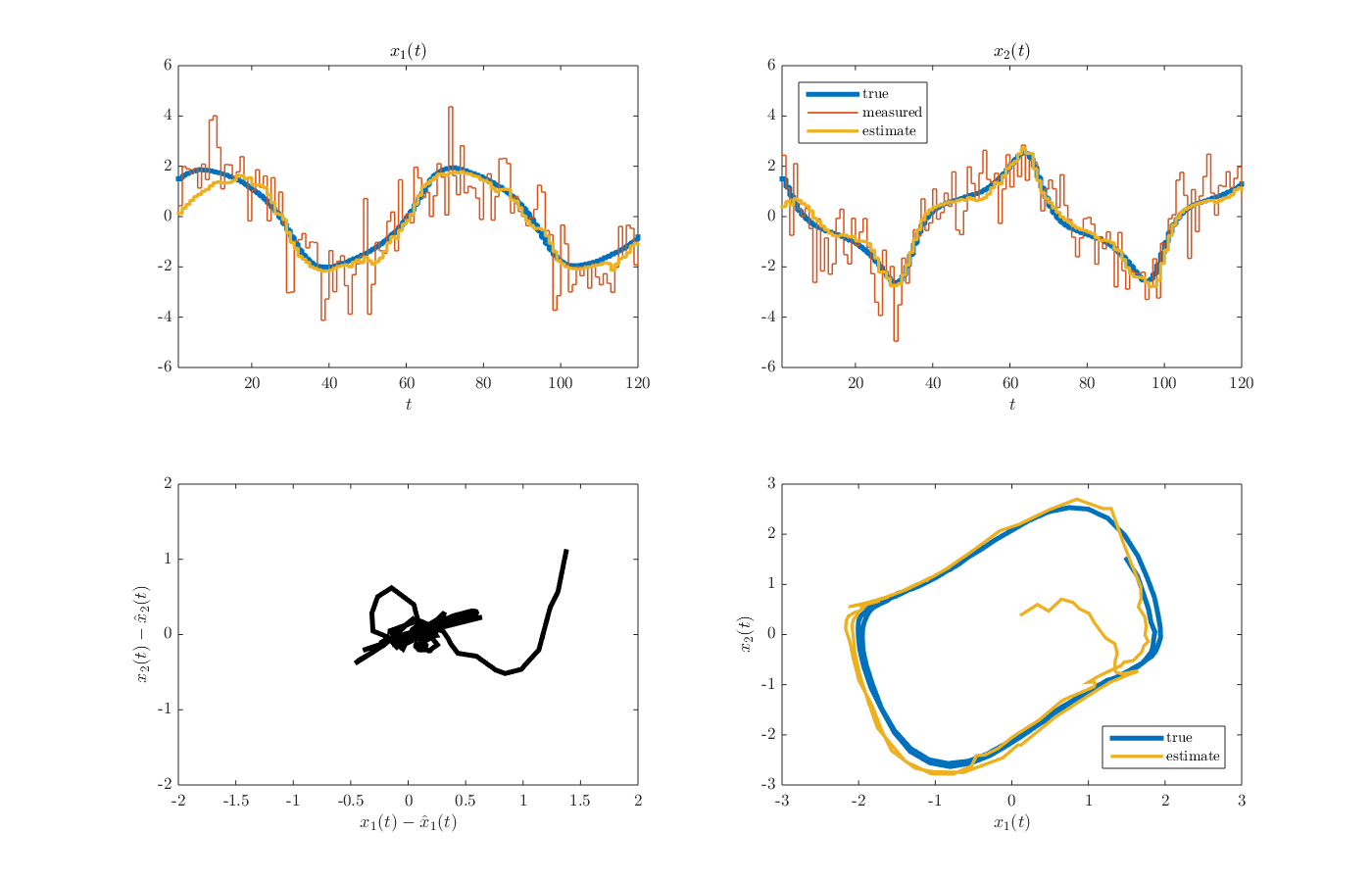
from the MATLAB command window. The arguments here (i.e., \(1.5\)) are elements of the initial state vector. After the simulation is finished, the results should appear as a structure named d in the MATLAB workspace. A figure summarizing the results, including the state and control input trajectories, can be produced using the function plot_results_NMHE.m by executing the command
plot_results_NMHE(d)
from the MATLAB command window. The resulting figure is given below.
-
Risbeck, M. J., & Rawlings, J. B. (2016). MPCTools: Nonlinear model predictive control tools for CasADi. ↩
-
Andersson, J. A., Gillis, J., Horn, G., Rawlings, J. B., & Diehl, M. (2018). CasADi: a software framework for nonlinear optimization and optimal control. Mathematical Programming Computation, 1-36. ↩
-
Wächter, A., & Biegler, L. T. (2006). On the implementation of an interior-point filter line-search algorithm for large-scale nonlinear programming. Mathematical programming, 106(1), 25-57. ↩
Leave a Comment