Model-based parameter estimation (with measurement noise) in MATLAB using CasADi

In this post we will attempt to create model-based parameter estimation (MBPE) code in MATLAB using CasADi. In particular, we will try to replicate some of the results of Bonilla et al. (2010)¹. We will need MATLAB and CasADi² (a free Python/MATLAB toolbox for nonlinear optimization and numerical optimal control). From CasADi we will call Ipopt³ for solving the resulting nonlinear optimization problems. You can download the code created in this post here: MBPE_meas_noise_CasADi.m.

We consider the following MBPE formulation, where the dynamics is affine in the parameters:

\[\begin{aligned} \text{minimize} & \quad \int_{0}^{T_{\text{exp}}}{\left\lVert x(t) - y(t) \right\rVert^2_Q} dt \\ \text{subject to} & \quad \text{for } t \in [0, T_{\text{exp}}]: \\ & \qquad \dot{x}(t) = f(x(t),u(t)) + g(x(t),u(t))p \\ & \qquad x(t) \in \mathbb{X} \\ & \quad p \in \mathbb{P}, \end{aligned}\]

where \(x \in \mathbb{R}^{n_x}\) is the state, \(p \in \mathbb{R}^{n_p}\) is the vector of parameters to be estimated, \(T_{\text{exp}}\) is the experiment horizon (length of recorded measurements in time units), \(Q\) is a matrix penalizing the mismatch between the state and measurements, \(f(\cdot)\) and \(g(\cdot)\) are functions representing the dynamics, \(y \in \mathbb{R}^{n_y}\) is the measurement of state \(x\), \(u \in \mathbb{R}^{n_u}\) is the recorded values of control input (if present), while \(\mathbb{X}\) and \(\mathbb{P}\) are sets representing constraints on the state and parameters, respectively.

We take the following system as an example:

\[\begin{aligned} \dot{x}_1(t) & = x_2(t)\\ \dot{x}_2(t) & = -p \cdot x_1(t), \end{aligned}\]

where \(x_1 \in \mathbb{R}\) and \(x_2 \in \mathbb{R}\) are the state variables, while \(p \in \mathbb{R}\) is the parameter to be estimated.

We specify various parameters and pre-allocate memory for the signals as follows:

function d = build_setup()
    
    % sampling time (in time units)
    d.p.T_s = 0.1;
    
    % experiment horizon (in time units)
    d.p.T_exp = 10;
    
    % experiment horizon (in time steps)
    d.p.k_exp = ceil(d.p.T_exp/d.p.T_s);
    
    % true parameter
    d.p.p_true = 10;
    
    % parameter scaling
    d.p.p_scale = 1;
    
    % parameter guess
    d.p.p_guess = 4;
    
    % state dimension
    d.p.n_x = 2;
    
    % parameter dimension
    d.p.n_p = 1;
    
    % measurement noise dimension
    d.p.n_v = 2;
    
    % memory preallocation for state trajectory
    d.s.x = NaN(d.p.n_x,d.p.k_exp);
    
    % initial state
    d.p.x0 = [0;1];
    d.s.x(:,1) = d.p.x0;
    
    % measurement noise standard deviations
    d.p.sigma_v = [0.1 0.1]';
    
    % set random number generator seed to 0
    % for repeatability
    rng(0)
    
    % measurement noise signal
    d.s.v = diag(d.p.sigma_v)*randn(d.p.n_v, d.p.k_exp);
    
    % matrix penalizing mismatch between state and measurement
    d.p.Q = eye(d.p.n_x);
    
end

Note that we use here values for the true parameter, sampling time, and experiment horizon that are different than what is used in Bonilla et al. (2010)¹, thus results will be slightly different overall.

We can define the dynamics as a CasADi function as follows:

function d = define_dynamics(d)
    
    import casadi.*
    
    % state variables
    x1  = MX.sym('x1');
    x2  = MX.sym('x2');
    
    % state variables vector
    states = [x1;x2];
    
    % parameters
    p  = MX.sym('p');
    
    % parameters vector
    params = p;
    
    % dynamics
    x_dot = [x2;-x1*p];
    
    % dynamics as a CasAdi function
    d.c.f = Function('f',{states,params},{x_dot});
    
    % record states and variables CasAdi objects
    d.c.states = states;
    d.c.params = params;
    
end

We can create a simulator object, that will act as the plant within the simulation, as follows:

function d = create_simulator(d)
    
    import casadi.*
    
    % create RK4 integrator
    k1 = d.c.f(d.c.states,d.c.params);
    k2 = d.c.f(d.c.states + (d.p.T_s/2)*k1,d.c.params);
    k3 = d.c.f(d.c.states + (d.p.T_s/2)*k2,d.c.params);
    k4 = d.c.f(d.c.states + d.p.T_s*k3,d.c.params);
    
    states_final = (d.p.T_s/6)*(k1 + 2*k2 + 2*k3 + k4);
    
    % create a function conducts one-step ahead simulation
    % from the current state
    d.c.Fflow = Function('Fflow',{d.c.states, d.c.params},{states_final});
    
end

We simulate the system using the following code, which approximates an experiment for recording the measurements on system state:

function d = simulate_system(d)
    
    % simulate system with the true parameter
    for k = 1:d.p.k_exp-1
        
        d.s.x(:,k+1) = d.s.x(:,k) + ...
            full(d.c.Fflow(d.s.x(:,k),d.p.p_true));
        
    end
    
    % create measurement trajectory by adding
    % measurement noise to the state trajectory
    d.s.y = d.s.x + d.s.v;
    
end

Finally, we can implement the original MBPE formulation as follows:

function d = solve_MBPE_original(d,p_guess)
    
    import casadi.*
    
    opti = casadi.Opti();
    
    % measurement trajectory
    y = d.s.y;
    
    % define state trajectory as decision variable
    x = opti.variable(d.p.n_x,d.p.k_exp);
    
    % define parameters as decision variable
    p = opti.variable(d.p.n_p,1);
    
    % initialize objective function
    J = 0;
    
    % construct state trajectory by simulating the system
    % as a function of parameters
    for k = 1:d.p.k_exp-1
        
        % simulate one step forward
        x_plus = x(:,k) + d.c.Fflow(x(:,k),p.*d.p.p_scale);
        
        % ensure continuity of state trajectory
        % (i.e., direct multiple shooting)
        opti.subject_to(x(:,k+1) == x_plus)
        
    end
    
    for k = 1:d.p.k_exp
        
        % add penalization of mismatch between
        % state and measurement to the objective function
        J = J + (x(:,k) - y(:,k))'*d.p.Q*(x(:,k) - y(:,k));
        
    end
    
    % configure solver options
    opti.solver('ipopt')
    p_opts = struct('expand',true);
    s_opts = struct('max_iter',100);
    opti.solver('ipopt',p_opts,s_opts);
    
    % set initial guess for parameters
    opti.set_initial(p,p_guess./d.p.p_scale);
    
    % set J as the objective function
    opti.minimize(J)
    
    try
        
        % attempt to solve the optimization problem
        sol = opti.solve();
        
        % undo scaling and record solution as the
        % parameter estimate
        d.p.p_hat_MBPE_original = sol.value(p).*d.p.p_scale;
        
    catch
        
        % give warning if the problem was not
        % successfully solved
        warning('problem during optimization!')
        
    end
    
end

If the above pieces are integrated and executed, we find that the optimization problem is successfully solved, and the solution is found as \(5.3\), although the true parameter value is \(10\). As explained in Bonilla et al. (2010)¹, this is due to MBPE formulation having a nonconvex objective function. 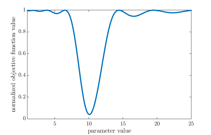This can be clearly seen by plotting the objective function values (which can be obtained by solving the original MBPE problem with the parameter fixed to a value, for a set of values): MBPE with measurement noise using CasADi, results

We thus see why the MBPE formulation we created above yielded a parameter estimate value of \(5.3\) that is far-off from the true value of \(10\): Starting from an initial guess of \(4\), the optimization procedure is getting stuck at a local minimum. Bonilla et al. (2010)¹ propose a remedy that is formulated as follows:

\[\begin{aligned} \text{minimize} & \quad \int_{0}^{T_{\text{exp}}}{\frac{1}{\lambda} \left\lVert x(t) - y(t) \right\rVert^2_Q + \frac{1}{1 - \lambda}\left\lVert x_c(t) - x(t) \right\rVert^2_Q} dt \\ \text{subject to} & \quad \text{for } t \in [0, T_{\text{exp}}]: \\ & \qquad \dot{x}_c(t) = f(x(t),u(t)) + g(x(t),u(t))p \\ & \qquad x_c(t) \in \mathbb{X} \\ & \quad p \in \mathbb{P}, \end{aligned}\]

where \(\lambda\) is a homotopy parameter and \(x_c(t)\) is a pseudo state. Using \(\lambda=1\) yields the original MBPE itself, while using \(\lambda=0\) yields a convex approximation of the original MBPE:

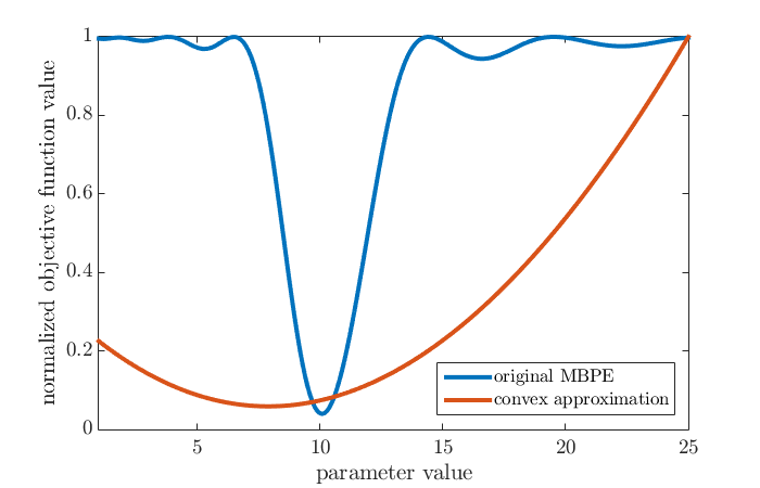
\[\begin{aligned} \text{minimize} & \quad \int_{0}^{T_{\text{exp}}}{\left\lVert x_c(t) - y(t) \right\rVert^2_Q} dt \\ \text{subject to} & \quad \text{for } t \in [0, T_{\text{exp}}]: \\ & \qquad \dot{x}_c(t) = f(y(t),u(t)) + g(y(t),u(t))p \\ & \qquad x_c(t) \in \mathbb{X} \\ & \quad p \in \mathbb{P}. \end{aligned}\]

It is thus possible to find a good initial guess for the original MBPE by solving the convex approximation, which yields a parameter estimate of \(7.9\). When this value is used as initial guess for the original problem, we obtain a parameter estimate of \(10.1\), which is fairly close to the true value of \(10\).

To see why solving the convex approximation can potentially lead to a good initial guess for the original problem, we can plot the objective function values original MBPE together with those of the convex approximation (which can be obtained by solving the convex approximation with the parameter fixed to a value, for a set of values): MBPE with measurement noise using CasADi, results

All pieces are integrated in the function MBPE_meas_noise_CasADi.m, which can be run by executing the command

d = MBPE_meas_noise_CasADi()

from the MATLAB command window. After the MBPE procedure is finished, the results should appear as a structure named d in the MATLAB workspace.

Bonilla, J., Diehl, M., Logist, F., De Moor, B., & Van Impe, J. F. (2010). A convexity-based homotopy method for nonlinear optimization in model predictive control. Optimal Control Applications and Methods, 31(5), 393-414. ↩ ↩² ↩³ ↩⁴
Andersson, J. A., Gillis, J., Horn, G., Rawlings, J. B., & Diehl, M. (2018). CasADi: a software framework for nonlinear optimization and optimal control. Mathematical Programming Computation, 1-36. ↩
Wächter, A., & Biegler, L. T. (2006). On the implementation of an interior-point filter line-search algorithm for large-scale nonlinear programming. Mathematical programming, 106(1), 25-57. ↩

Işık İlber Sırmatel

Model-based parameter estimation (with measurement noise) in MATLAB using CasADi

Leave a Comment

You May Also Enjoy

A Coverage Control-Based Idle Vehicle Rebalancing Approach for Autonomous Mobility-on-Demand Systems

Nonlinear model predictive control of large-scale urban road networks via average speed control

Idle-vehicle rebalancing coverage control for ride-sourcing systems

Modeling, estimation, and control in large-scale urban road networks with remaining travel distance dynamics